CFD Analysis of a Stratified Storage System

The new OpenFOAM® investigation buoyant driven flows created during summer 2020

After the website release in June 2020, I decided to investigate an old topic called »stratified storage system«. A few years ago (around 2014), I tried to simulate the layering inside a heating storage tank without success. Since I gained a lot of knowledge in the last few years, I re-investigate the topic as I also do have a new working station (Threadripper Gen. 3 with 32 cores), which allows me to create a more complex and realistic system. A stratified vessel system commonly uses simple physics to store hot water intelligence. The vessel works as follows: Hot new air is inserted in the bottom region of the storage tank. The hot injected water enters a subsystem that allows infused water to flow upwards the vessel - due to the buoyancy effect - until it reaches the correct temperature region (height). In that height, it leaves the subsystem in the vessel and enters the storage tank via the port.

The created geometry is an arbitrary design, hopefully working as expected. One can search on the web to see more advanced systems. I was surprised that there are some real inadequate vessels available one can purchase. If you look at the design, you definitely will say: "No way this is not working as a stratified system.". Nevertheless, as these systems exist, they are probably people who install such inadequate systems.

The vessel generated in this post has a volume of 3500 liters. In the CFD analysis, I suppose that the circulation pump has a volumetric flow rate of 0.25 l/s, that equals to 900l/h. Thus, within one hour, the circulation pump can exchange 1/3 of the volume inside the vessel. The assumed volumetric flow rate might be too large or too low. However, we will see the results in the analysis.

Warning: Undefined array key 1 in /var/www/web610/html/2021/modules/mod_downloader/tmpl/default.php on line 19

Warning: Undefined array key 1 in /var/www/web610/html/2021/modules/mod_downloader/tmpl/default.php on line 19

Geometry Preparation using SALOME and the Shaper Module

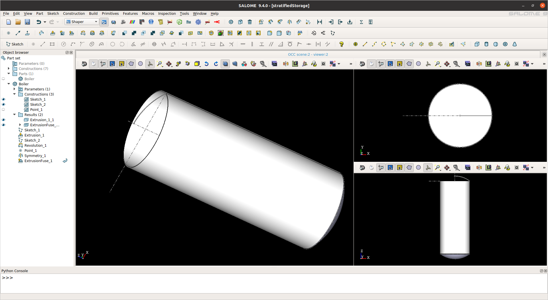
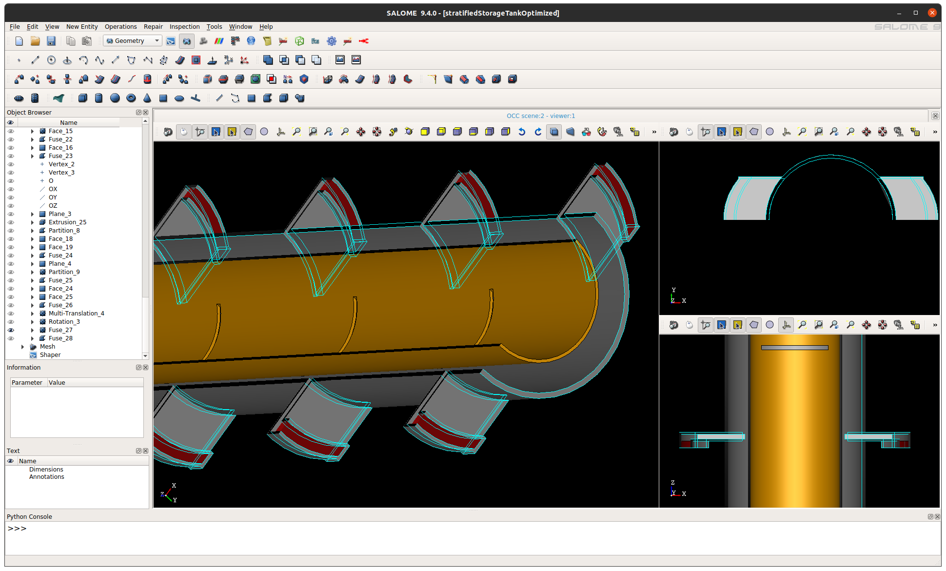
For the CAD modeling, I used the Salome version 9.4.0 and the Shaper module. For the storage tank, I decided to make a more advanced model in terms of feature elements such as the standing legs, more nozzles, a revision flange, etc. The starting point was the extrusion of the outer shell, followed by the top part of the storage system. After the base model was created, I started to build the pedestal of the storage tank. Here, I extruded always until the bottom of the tank. To do so, one can use the extrusion tool and select the »extrusion to« option, marked in red in the picture below.

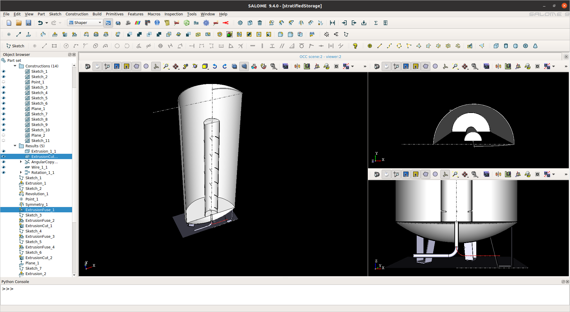
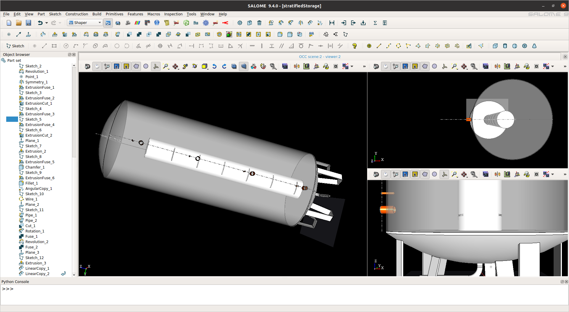
As one can see, I already added the intake port system. A more detailed view is given in the picture below. Subsequently, I created the inlet pipe system. This pipe will carry the hot water into the vessel's subsystem. For this purpose, I used the capability of Salome to extrude a sketch along a path. The following »YouTube video« will guide you through the essential steps for this action. The subsystem inside the vessel is needed to allow the hot water, that is entering the storage tank, to rise to the correct temperature height related to the buoyancy force without disturbing the temperature layering inside the vessel. Therefore, the subsystem itself depends on an empty pipe, including different ports at different heigths. Finally, I designed four outlet ports and four temperature ports (1/2"), respectively. For a more advanced and impressive visualization for the numerical results, I created a revision flange in addition. The complete CAD model is depicted in the right picture given below. The STEP file can be downloaded at the end of this section.

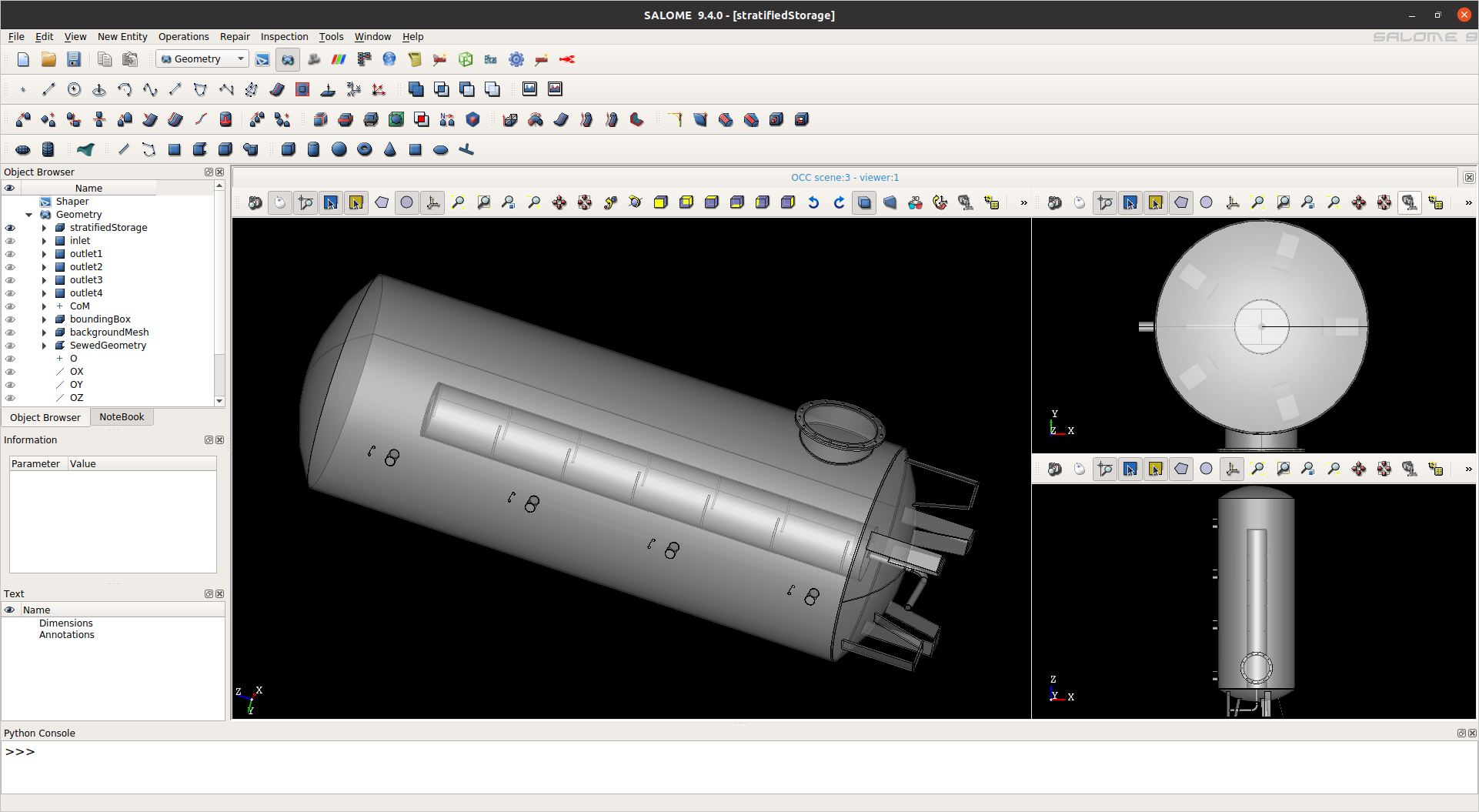
It should be evident that the design is not optimized or does play any relevance for our lives. Right now, while looking at the pictures above, I realize that the outlet nozzles might be in a better position if we would turn them, e.g., by 90°. That's because I would expect that, if, for example, we use the lowest outlet port, it might happen that we directly suck out the hot water which is carried into the vessel. However, this will only occur if the volumetric flow rate is too large. Nevertheless, while checking the web, there are plenty of possibilities and ideas on how to create such a vessel. However, the design of the geometrical aspects should be - due to the physics - always identical:

• Cross section extension to lower the speed of the fluid
• Due to the first point, enable a laminar flow everywhere
• Blocking jet streams and try reach a design that allows the inserted hot water to go to the right height (with the corresponding temperature level)

Geometry Adaption for the CFD Analysis using Salome

Since the geometry was completed in the Shaper module, I exported it into the Geometry module. Here, I did the usual work such as adding patches for »inlet and outlet«, reducing the model for a CFD analysis to a single surface, create different patches for the surface meshing procedure, create the bounding box and enlarge it by, e.g., 1 % of size (this is important for snappyHexMesh), export everything to the Mesh module and created the background mesh (using the scaled bounding box). Finally, I made the surface triangulation of the watertight surface while adding the patches, which can be exported as a single STL file. As my favorite method in snappyHexMesh is using so-called region STL files, I copied each exported (single patch) STL file content into one. I want to mention that I use the hexahedral meshing process in Salome to generate the background mesh for snappyHexMesh; this is exported as *.unv file which can be converted to an OpenFOAM® mesh later on. You can check out how to create such a mesh in the »Training Videos« section of my website. By the way, you will also gain a lot of knowledge related to Salome and OpenFOAM® in general.

Finite Volume Meshing using SnappyHexMesh

After the pre-processing of the CAD model was performed and the background mesh was exported as an *.unv file, I am using a bash script that performs the following processes:

• Create the region STL and place it (copy it) to the correct location (constant/triSurface)
• Based on the single STL files, a bash script automatically creates the snappyHexMeshDict including all single regions
• Convert the *.unv mesh into an OpenFOAM® mesh (constant/polyMesh)

As I am a lazy guy, the first meshing can be started after seconds, and since, the first numerical mesh is present within a few minutes. It is worth mentioning that I do use bash scripts for the meshing purpose. The scripts will do a lot of work for me, such as cleaning the case, decomposing, running snappyHexMesh in parallel, reconstructing, renumbering, and so on. I do love the way I can control OpenFOAM® in the bash environment. It is fast, reliable, and easy to handle.

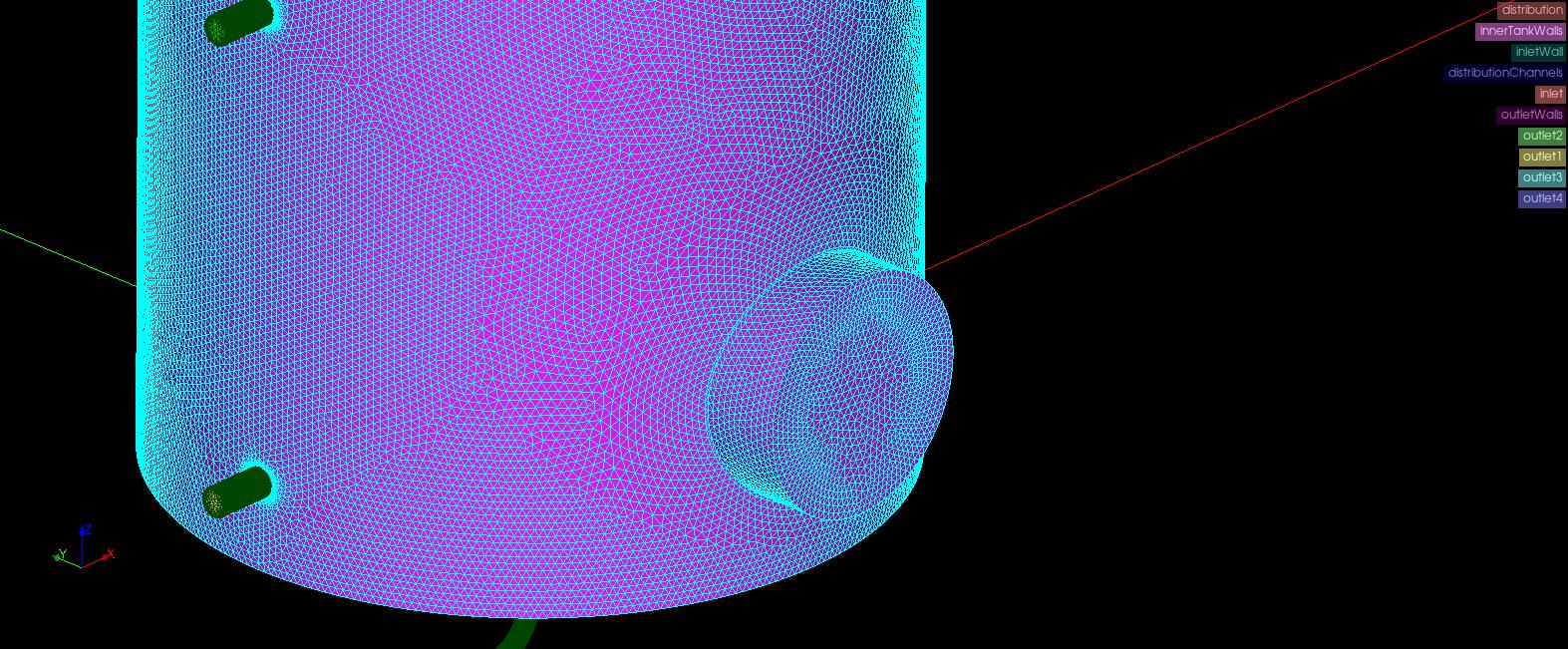
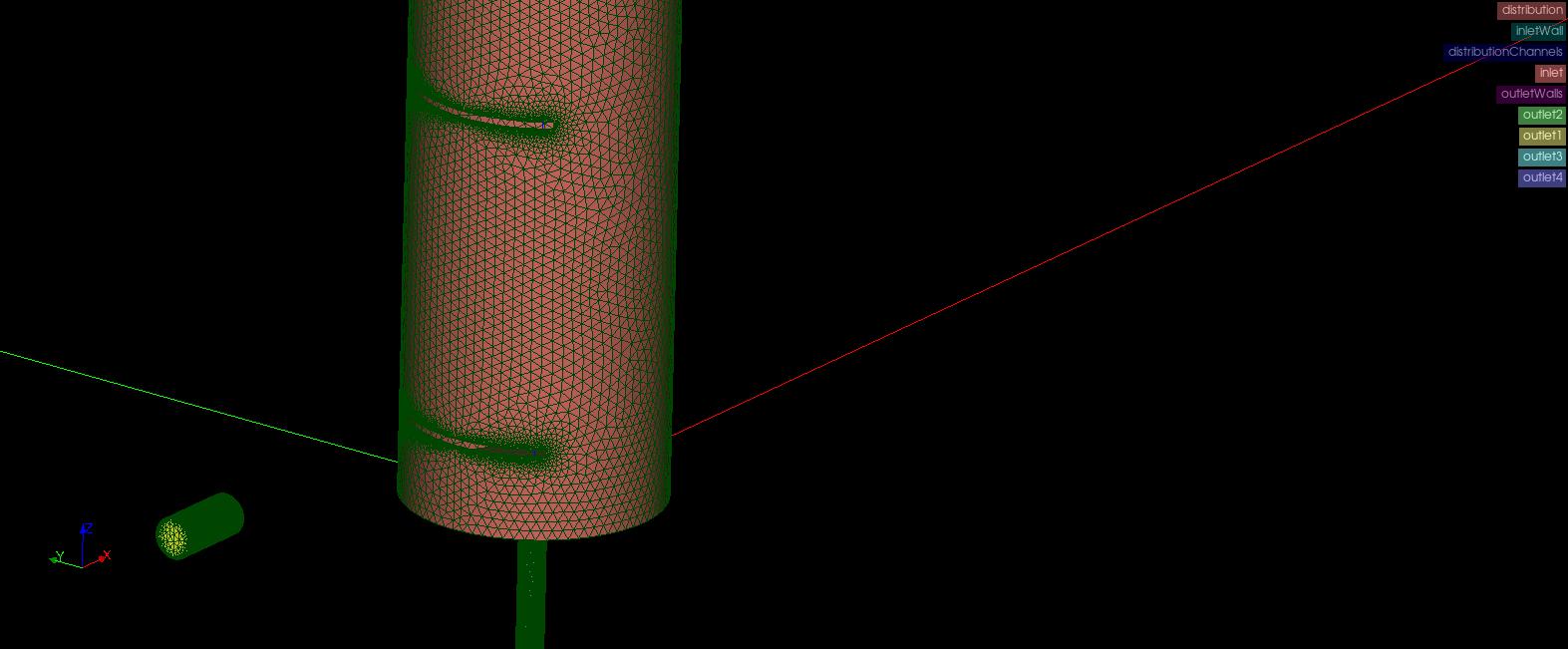
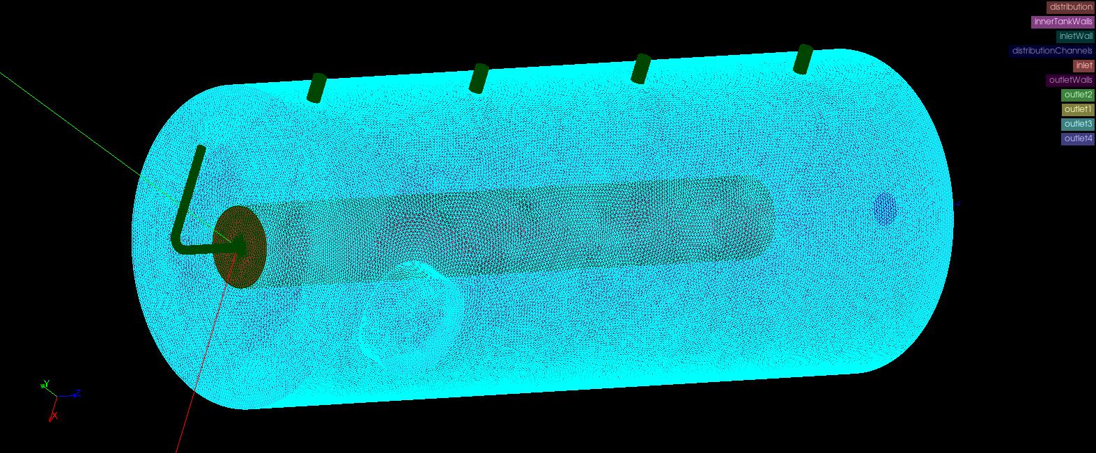
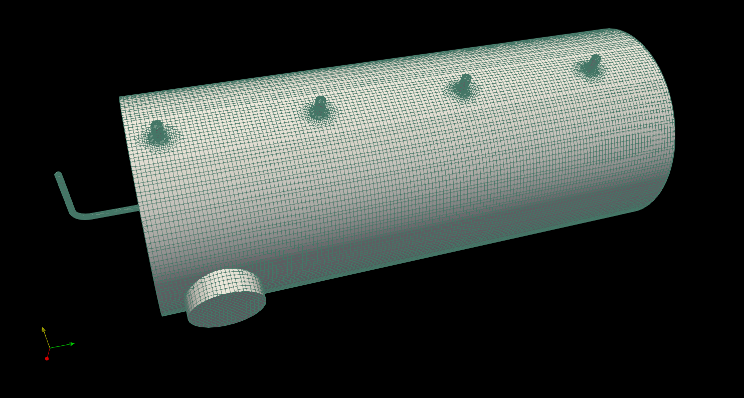
The pictures below show the numerical mesh that was used in the numerical analysis. After around ten minutes of optimization, I decided to keep the mesh while trying to keep the port in the subsystem cells as large as possible. We do have the smallest cells in the ports of the subsystem and, therefore, probably the most significant velocities. Hence, these cells will determine the time-step of the calculation. I want to mention that you might get trouble during the visualization of the mesh edges in the latest ParaView® version.

Note: If you force strange behavior of the edges, e.g., the surface seems to be transparent, and you see edges that should be hidden, you should play around with the value of the second (right one) »Polygon Offset Parameter«. You find the option in Edit » Settings » Render View.

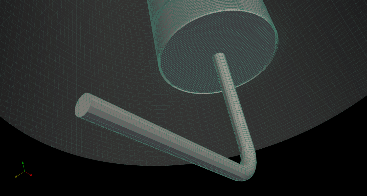
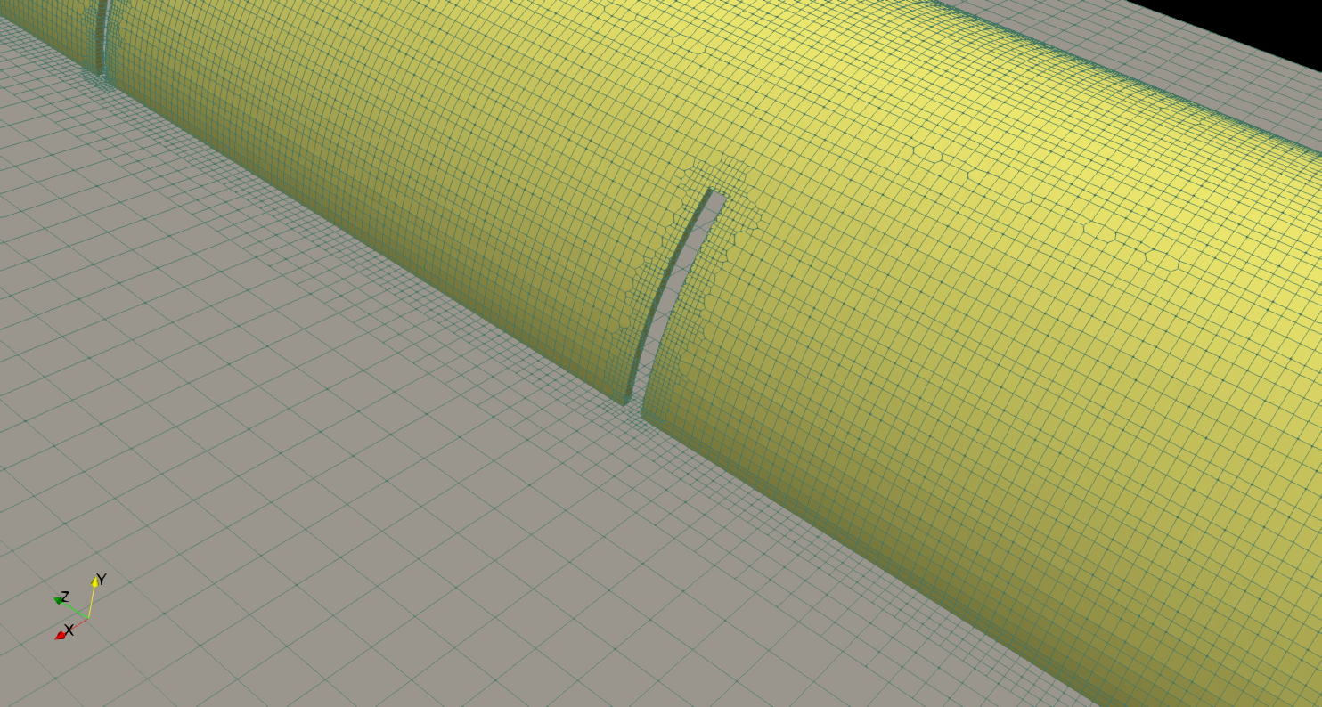
Boundary Conditions and CFD Set-up

For the numerical analysis, I decided to have a fixed flow rate at the inlet pipe system of 0.25 l/s. However, the energy of the water will change during time. Therefore, I used the »uniformFixedValue« boundary condition in order to enable the usage of the »function1« capability of OpenFOAM®. Doing so, we easily can set-up a table that sets the temperature to different values with respect to the corresponding time. In this example, I used the »table« functionality of the »function1«. The temperature of the water will change as follows:

• The initial temperature of the whole vessel is 15 °C
• For the first 60 s, the inlet temperature is 27 °C
• After that, the temperature is set to 37 °C for one more minute
• Subsequently, the temperature is again increased by 10 K to 47 °C for three minutes
• Then, for five minutes the temperature is 77 °C
• Which is followed by 92 °C for 20 minutes
• Afterward, the temperature is reduced to 58 °C for ten minutes
• And again increased to 62 °C for 15 minutes
• At last, water with 94 °C is added for five more minutes

Summing up, we do have a transient calculation of 3600 seconds. During that period, the water temperature is changed according to the list given above. Especially in the last 30 minutes, as the temperature is varied up and down. Due to the buoyancy effect, and the subsystem, the added water should be correctly layered into the right position. I believe 58 °C, 62 °C, and 94 °C will demonstrate if the design will work.

Additionally, a heat transfer at the surface of the vessel was applied. The vessel sheet thickness is assumed to be four millimeters with a heat conductivity of 25 W/m/K. Besides, the tank has a 100 mm isolation (0.035 W/m/K). The room temperature (far-field temperature) is set to 15 °C (initial temperature of the tank), and a heat transfer coefficient (HTC) of 10 W/m²/K was assumed. The pressure is set to 1.5 bar(a), which will not influence the calculation (at the outlet, a »fixedMean« boundary condition was applied). The thermophysical properties are based on polynomials, which are presented and discussed in the »Temperature Depended Thermophysical Properties for Pure Water« blog. I am aware that the polynomial data are for atmospheric pressure, but I don't believe this will influence the system in its fundamental physics.

A standard numerical solver was used (buoyantPimpleFoam) and the schemes were set to first-order Gauss upwind. For a more accurate calculation, one should switch to higher-order schemes. However, as this is just a fun and demonstration case for free-buoyancy driven flows, I decided to keep the Gauss upwind scheme for all investigations.

CFD Results & Numerical Analysis

After the OpenFOAM® case was set up as described above, the case was run in parallel (25 cores) on my local machine using the AMD Threadripper 3970X CPU. The time-step was adjusted related to the Courant number (Co). The maximal limit was set to Co = 0.9 in the beginning. However, this would lead to a calculation time of 26 days. Hence, I updated the solver settings to use the PIMPLE algorithm with weak residual controls and set the maximal allowed Courant number to 20. Therefore, the computational effort reduced to around 28 hours for a total calculation time of around 45 minutes; I did not investigate into the full 60 minutes and additionally, the advanced boundary condition - time-dependent inlet temperature - could be neglected at all.

I compared both calculations, Co = 0.9 and Co = 20, at an identical time (approximately 300 s), with the conclusion that both setups are similar. Nevertheless, it was evident that we do lose some transient features if we go beyond Co = 1. Therefore, the contour plots were different but in a similar physical meaning.

The numerical data were analyzed using the post-processing software ParaView®. The video below gives an insight into the thermal-flow behavior of a complete cold storage tank during the first loading step. As one can see, in the beginning, the hot water rises inside the sub-system based on the velocity and buoyancy effect. Here, the main driving force is the velocity impulse from the inlet system of the storage tank. However, the warm fluid enters the sub-system at the top and moves further up (as expected). Unfortunately, the flow pattern of the hot water forces the cold water to enter into the sub-system; re-circulation areas are the driving force. Hence, a classical cold/warm mixing structure develops inside the sub-system. After a couple of minutes, the sub-system behaves like a well-designed mixing system. The outcome is that the whole storage tank heats-up uniformly rather than separated in layers.

Thus, the design I made failed the expected behavior and is not appropriate for such systems. After the analysis of the numerical data, I first re-run the calculation using half of the volume rate. However, the analysis showed, that similar results are performed and the main problem is the cold-hot water mixing in the sub-system; the results are not shown in the blog.

After these two investigations, I thought that the channels of the sub-systems might be too small. The next video shows the extended channel sizes. As one can see, the situation does not change at all. We still do have the same phenomenon acting here. There is still a high mixing from hot and cold water right at the bottom of the sub-system. Compared to the small channels, the mixing is even higher and the vessel gets even more uniformly heated rather than loaded based on the buoyancy effect.

As this example demonstrates, the physics inside a very »simple« geometry can be more complicated than expected during the design phase. Conclusion: The system is wrong designed to behave as a stratified storage system.

Optimization of the Stratified Storage System

After the numerical analysis, it is obvious that the design behaves wrong and the cold water should not enter the sub-system where the hot water is injected and rises to the corresponding height. If one does have more experience of fluid flows and geometry optimization, there are a few points that are obvious to change.

• The inlet velocity is too larger, hence, a diffusor including a perforated plate could slow down the fluid which will lead to a more smooth flow pattern (less vortexes)
• The sucking effect has to be stopped or at least decreased and hence, the sub-system should be re-investigated and optimized

The first point is clear. The inlet part was re-designed to include a diffusor (cross-section increase). It also consists of a perforated plate (this was not geometrically resolved, but a porous media assumption was used later on). The second point is a bit more tricky. Here, one can do a variety of improvements and changes. I decided to decouple the subsystem further. Hence, an additional shell was added (it is the orange pipe in the sub-system as depicted in the figures below). Therefore, three fluid regions appear. The outer liquid area (storage tank itself), the inner sub-system fluid region between the two sub-systems, and the fluid region represent the volume in which the fluid can rise due to the buoyancy effect. The CAD pictures below give more details of the design optimizations.

Furthermore, the channels from the sub-system to the central fluid region were newly designed to include flow directed channel systems. The port of these new channels points downward and inherits a perforated plate at the port (given in red in the right figure below). The red regions were modeled using a porous media assumption in the CFD analysis. The idea is that a higher pressure drop does not allow the fluid to enter the channels from the storage tank into the sub-system, and therefore, the mixing characteristic we found before should vanish.

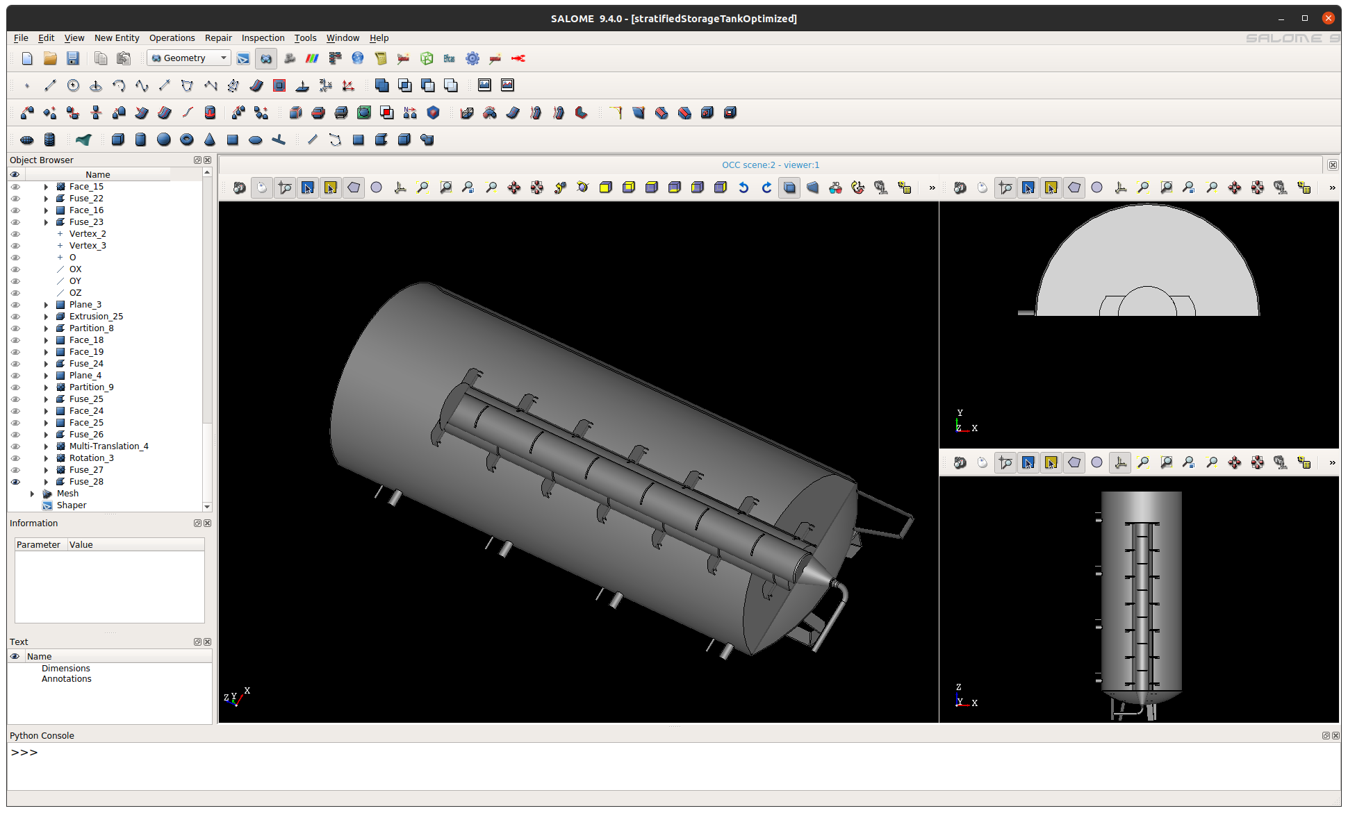
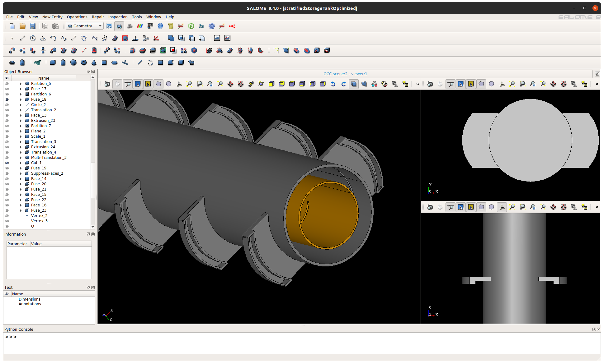
The set-up for the CFD calculation was kept identically compared to the first investigation. However, for the port channels and the perforated plate at the diffusor, a porous media assumption was used. Therefore, the »fvOptions« capability of OpenFOAM® was used to introduce a source/sink term to the momentum equation. For the porous media calculation, the »Darcy-Forchheimer« model was used with the following parameters:

The set-up for the CFD calculation was kept identically compared to the first investigation. However, for the port channels and the perforated plate at the diffusor, a porous media assumption was applied. Therefore, the »fvOptions« capability of OpenFOAM® was used to introduce a source/sink term (on the fly) to the momentum equation. For the porous media calculation, the »Darcy-Forchheimer« model was selected, and the following arbitrary parameters were set:

• For the perforated plate which is placed at the diffusor, a linear approximation was used (only Darcy) with D = 10000 defined in the z-direction. The x-, and y-direction were set to -1e6
• A similar set-up was used for the port outlets. However, here the Darcy coefficient was set to D = 5000

Commonly, these values are not notable. At the end of the simulation, I realized that these quantities should be increased to get a better contribution of the porous media onto the flow pattern. This is visible in the diffusor part. Here the flow stream is not uniformly distributed. There is a jet stream going still up.

The analysis of the numerical data was performed identically as before. However, now the flow pattern differs, as one can see in the video below. The mixing of the cold and warm water still occurs but not as significant as in the original geometry. After around 15 minutes (900 s) the layered temperature regions are obviously established. Sure, there are still a lot of improvements one can do here, e.g., extending the sub-system up to the top and play around the porous media properties. Nevertheless, the system behaves now as expected and the layering of different temperature regions occurs.

Conclusion: The investigation done in this blog shows how CFD and numerical studies can support the design phase - here, a storage system. Additionally, the CFD analysis gives more insight into the phenomena occurring inside a system. As a result of this, it is possible to optimize the design even before the device is built. I am personally a bit fascinated that this design behaves so differently in the first shot. I was expecting something different.

--
I hope you could get something out of this blog and that it was helpful for you.
Keep foaming & Glück Auf,
Tobias Holzmann