Darcy-Forchheimer Calculator

Estimate the Darcy-Forchheimer coefficients to model porous media in your simulation

The calculation is based on the

Select a calculation mode

Mass-Flow Rate

[kg/s]

Cross-Section Area

[m²]

Coefficient r

[Pa/m²]

Coefficient f

[kg/m³]

Velocity

[m/s]

Pressure Loss

[Pa]

Density of the fluid

[kg/m³]

Dynamic Viscosity of the fluid

[kg/m/s]

Length of porous zone

[m]

Darcy contribution D

[1/m²]

Forchheimer contribution F

[1/m]

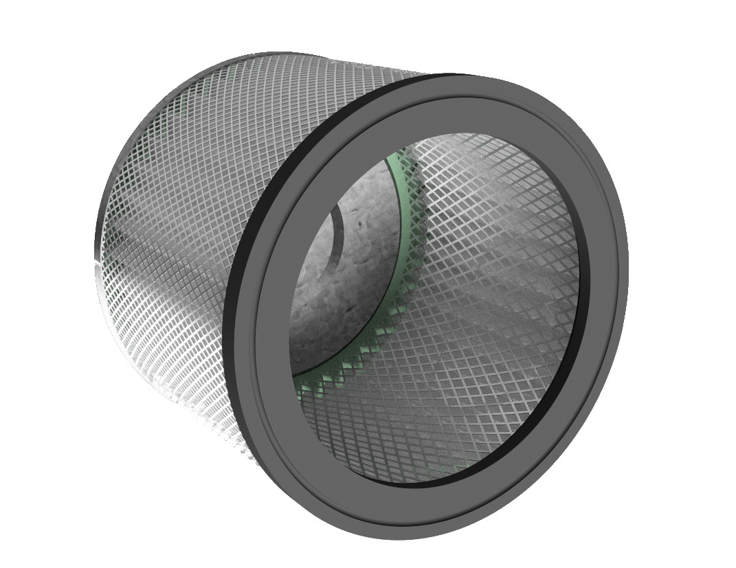
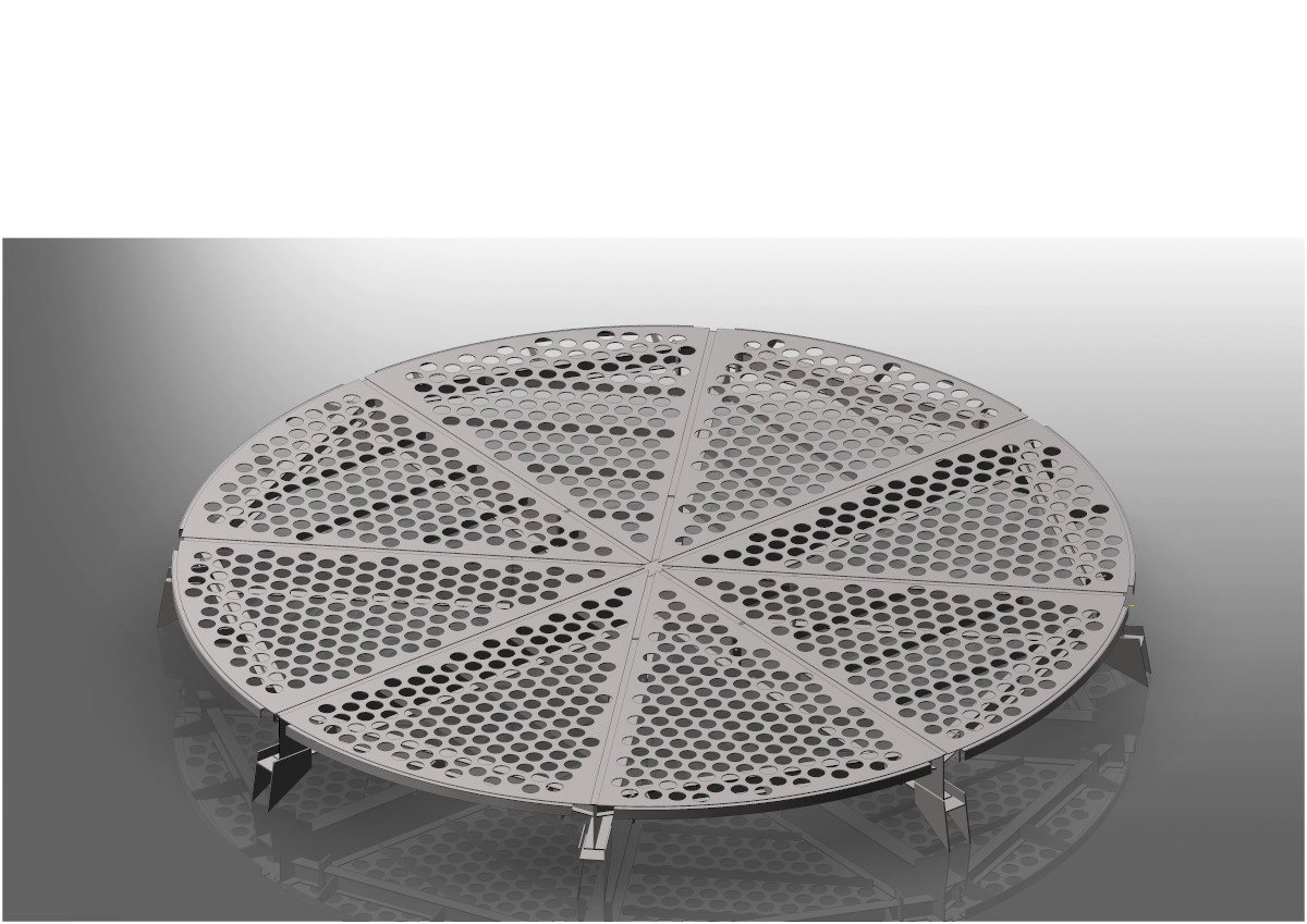
In many engineering applications, different objects can be inserted into the flow, such as honeycombs, perforated plates, and filters. The main effect on the flow of these objects is a pressure drop and, in most cases, an additional velocity direction correction. For example, through perforated plates with a large thickness or honeycombs, the fluid can only pass in one direction. However, for filters, a flow direction correction might happen or not. Nevertheless, the central aspect is the pressure drop in the fluid flow.

If we consider resolving each of these narrow channels, we will end up in a large mesh. Additionally, the time-step will reduce due to the small cells and the increase in velocity (Courant number definition). Hence, in computational fluid dynamics, we are modeling these zones with so-called »porosity models«. One of these models is the famous »Darcy-Forchheimer« or »Power Law« model. These models are commonly applied to a defined cell zone in which the momentum equation gets a new sink/source term.

The Darcy-Forchheimer model is a tensor model of rank 1. Hence, one can apply flow-directed pressure drops. The calculator created by Tobias can be used to estimate the model parameters for the Darcy-Forchheimer model. Based on the equation — given below — three different modes can be used.

Linear velocity-pressure drop relation (F = 0 » only Darcy contribution)
Parabolic velocity-pressure drop relation (D = 0 » only Forchheimer contribution)
A mixed formulation based on (1.) and (2.)

The choice of the calculation mode depends on the pressure-velocity relation of the porous media. In most cases, the parabolic velocity-pressure link is sufficient to reproduce the real pressure drop scenario of the obstacle.

\[\nabla p = \left(\mu \textbf{D} + \frac{1}{2}\rho \textbf{F} \textbf{U}\right)\textbf{U} ~~~~~\Longleftrightarrow~~~~~ \nabla p = \frac{\Delta p}{\Delta x} = r \textbf{U} + f \textbf{U}^2\]

Pictures from https://grabcad.com

From the expressions above, the following statements can be derived:

\[\nabla p = \left(\mu \textbf{D}\textbf{U} + \frac{1}{2}\rho \textbf{F} \textbf{U}^2\right) ~~~~~\Longleftrightarrow~~~~~ \nabla p = \frac{\Delta p}{\Delta x} = r \textbf{U} + f \textbf{U}^2\]

\[\mu \textbf{D}\textbf{U} \Longleftrightarrow r\textbf{U} ~~~~~ ~~~~~ \frac{1}{2}\rho \textbf{F} \textbf{U}^2 \Longleftrightarrow f \textbf{U}^2\]

\[\mu \textbf{D} = r ~~~~~ ~~~~~ \frac{1}{2}\rho \textbf{F} = f\]

\[\textbf{D} = \frac{r}{\mu} ~~~~~ ~~~~~ \textbf{F} = \frac{2f}{\rho}\]

Below one will find the calculator tool for estimating the parameters D and F. These parameters are vector quantities, hence, one can estimate different pressure drops for different directions. If one direction should block the flow, it is possible to set negative values or extremely large quantities such as 1e8. If one sets a negative number, it gets multiplied by the larges positive number and set as positive quantity in the model.