Gray Scott Model

An interesting two-equation model for different purposes

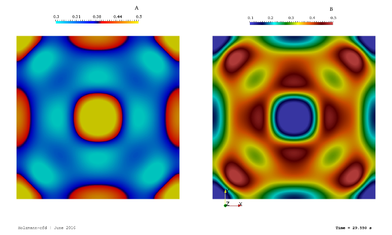
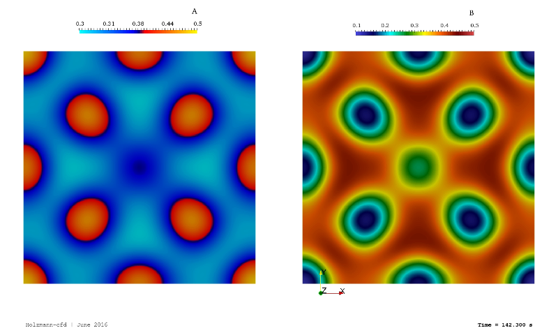
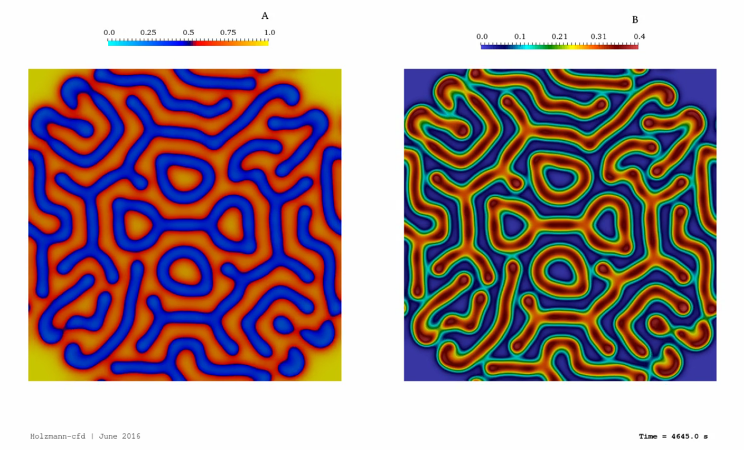
The Gray Scott Model is a reaction-diffusion model that uses two non-real species named A and B, which »react« and transform to each other. Due to the mathematical expression, both equations (for A and B) are coupled. The model is used mainly to investigate numerical schemes and is a playground for people who love to create beautiful fluid flows and flow-patterns. That is because the simple equations lead to interesting reaction patterns only if we change the model parameters slightly. Tobias investigated into that model and its implementation during his Ph.D. study at the Montanuniversität Leoben. Here, in the lecture »numerical mathematics II«, the object was to implement this model into the Matlab application. However, Tobias decided to implement it also into the OpenFOAM environment using different approaches such as explicit and implicit. Thus, the repository will give one information about the differences between the two methods, and one can investigate the speed and accuracy and other parameters as well.

The Gray Scott Model is an interesting topic to investigate and learn about numerics

If one is interested in that model in more detail, feel free to visit the following sites:

The equations that describe the Gray Scott model are extended by Tobias. Thus, the advective term was incorporated. Therefore, the implemented equations are given as:

\[\frac{\partial A}{\partial t} + \nabla \bullet (\textbf{U} A)= D_a \nabla \bullet (\nabla A) - AB^2 + f(1-A) ~~~~ (1)\]

\[\frac{\partial B}{\partial t} + \nabla \bullet (\textbf{U} B) = D_b \nabla \bullet (\nabla B) + AB^2 - (f + k)B ~~~~ (2)\]

The characteristics of both equations are:

In equation (1), the quantity »A« is linear in each term
In equation (2), the unknown »B« is non-linear in the second term on the right-hand side and linear in all other terms
The second term of each equation represents the coupling term (A + 2B reacts to 3B)
The last term of each equation represents a source or sink term
In equation (1) a continuous feeding rate (f) is present
In equation (2) a continuous reduction/killing rate (k) is present

A detailed derivation of the matrix one has to solver for A and B can be found in the »The Book & Publications« section of the website. Tobias tries to translate the manuscript into English, once he has a bit more time for such kind of work.

Git

Github URL: https://github.com/shor-ty/GrayScottModel
Build by Tobias Holzmann
Support the work of Tobias Holzmann